BDMM-Prime for Macroevolution
This tutorial assumes that you have already gained some experience using BEAST2. If you have not already done so, we recommend first completing the following tutorials:
Background
BDMM-Prime is a package written for flexible phylodynamic inference. It combines the functionality of multiple other packages, including the BDMM, BDSKY and SA packages, and can be applied to a wide range of scenarios in epidemiology and macroevolution. Due to the flexibility and the large variety of ways in which model parameters can be combined using BDMM-Prime there’s more options to consider when setting up your analysis.
This tutorial walks you through some examples of how the package can be applied in macroevolution. For an example in epidemiology see the BDMM-Prime package website.
The data
We’ll use a published dataset of aminotes that has been used previously to explore the early evolution of this group.
The data comprises 294 characters for 70 fossils, as well as their age and locality information, spanning ~70 myr from the late Carboniferous to the mid Triassic. The specimens can be categorised into three broad geographic areas associated with the north, mid, and south of the supercontinent Pangea, corresponding approximately to what would be known today as Eurasia, North America, and South Africa.
Installing the BDMM-Prime package
The first thing we need to do is install the BDMM-Prime package. This package is not yet listed in the Package Manager in BEAUTi, so we need to install it using the package URL.
- Open BEAUTi and go to File > Manage Packages.
- Select ‘Package repositories’ at the bottom of this window. This will open the ‘Package Repository Manager’.
- At the bottom click ‘Add URL’ and enter the following address: https://tgvaughan.github.io/BDMM-Prime/package.xml
After you click ‘OK’ your window should look like this:
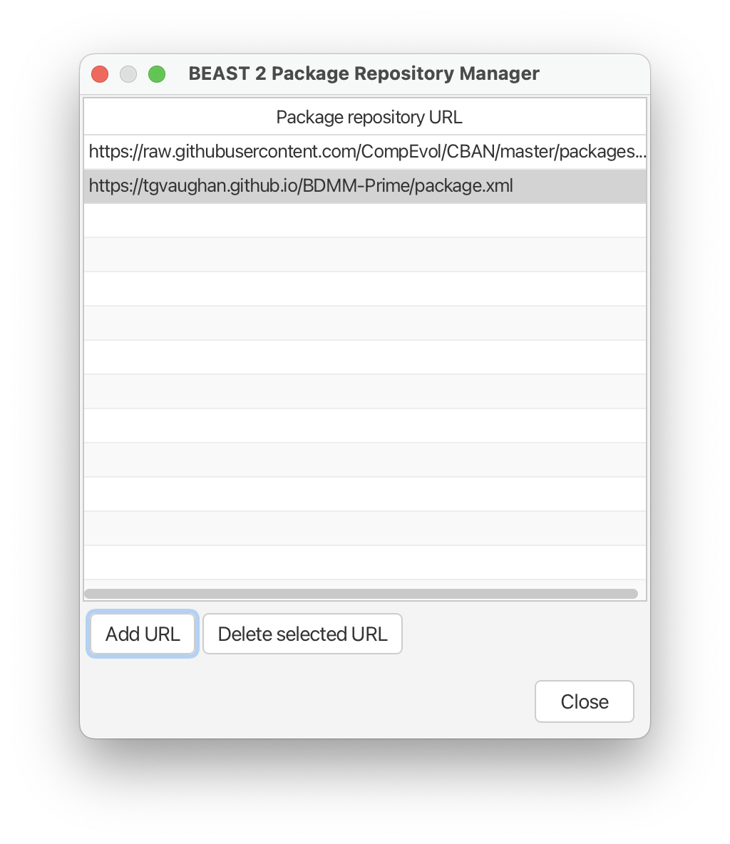
- Click ‘Close’. The BDMM-Prime package should now appear in your list of available packages.
- Select the BDMM-Prime package and click ‘Install/Upgrade’ at the bottom of the window. This should bring up a message that confirms the package has been successfully installed.
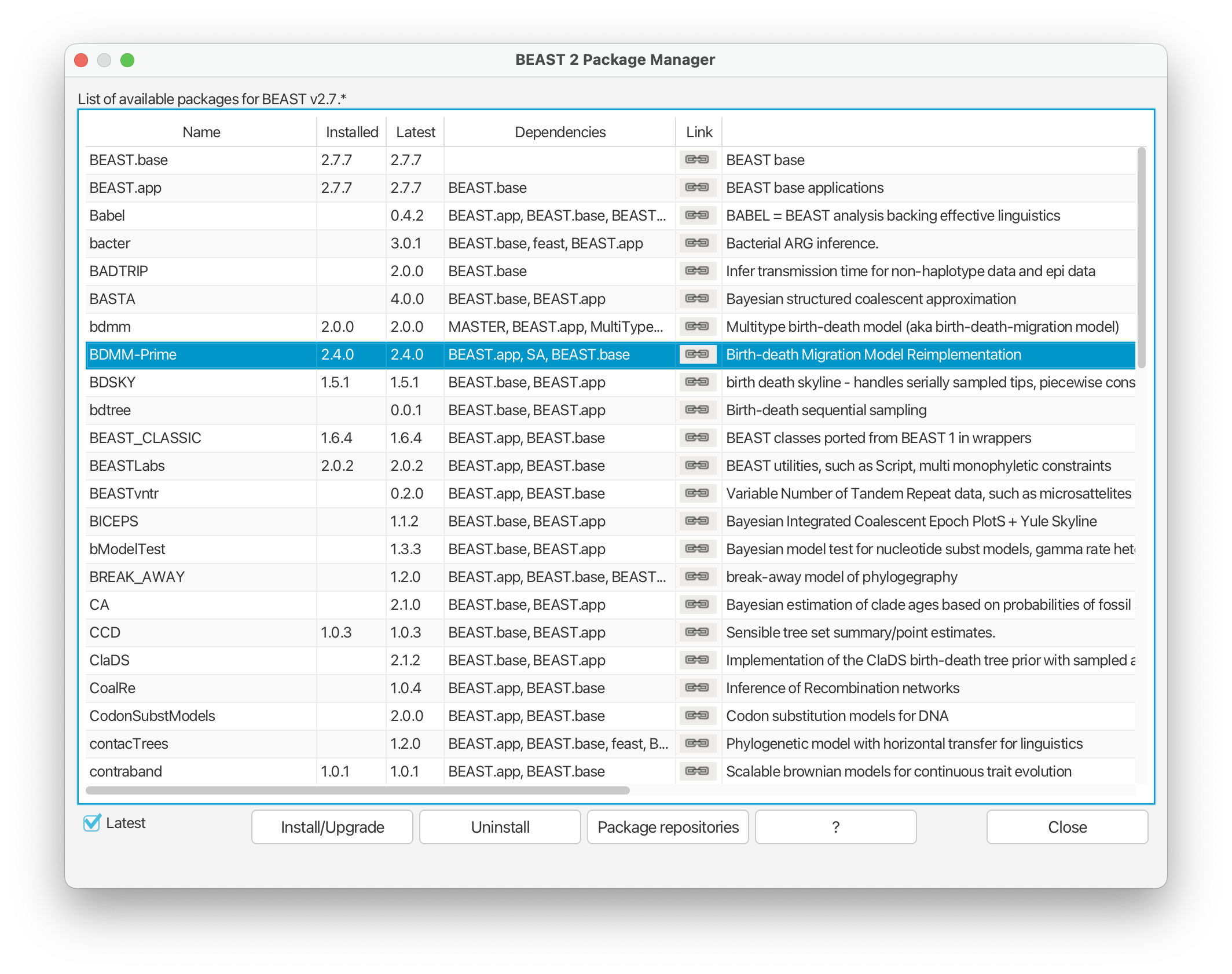
- If you haven’t done so already, you will also need to install the MM package for models of morphological evolution to complete this tutorial. This package should already appear on the same list in the Package Manager. You just need to click ‘Install/Upgrade’.
Restart BEAUTi to set up an analysis using BDMM-Prime.
The Partitions panel
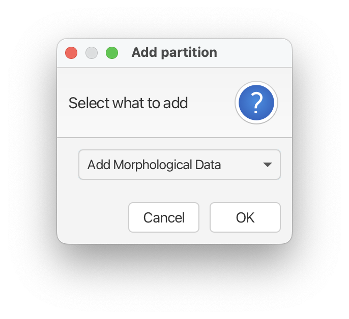
Download the nexus file associated with this tutorial. To input your data into BEAUTi, download the nexus file and either drag and drop the file into the Partitions panel and select ‘Add Morphological Data’ and then ‘OK’ or go to File > ‘Add Morphological Data’.
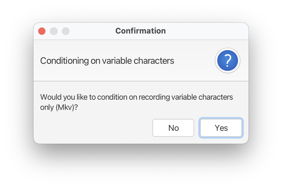
This will bring up a window that asks, “Would you like to condition of recording variable characters only (Mkv)?” Click ‘Yes’. Since we typically don’t collect non-variable morphological characters this option makes sense for our dataset.
Your BEAUTi window should now look like this:
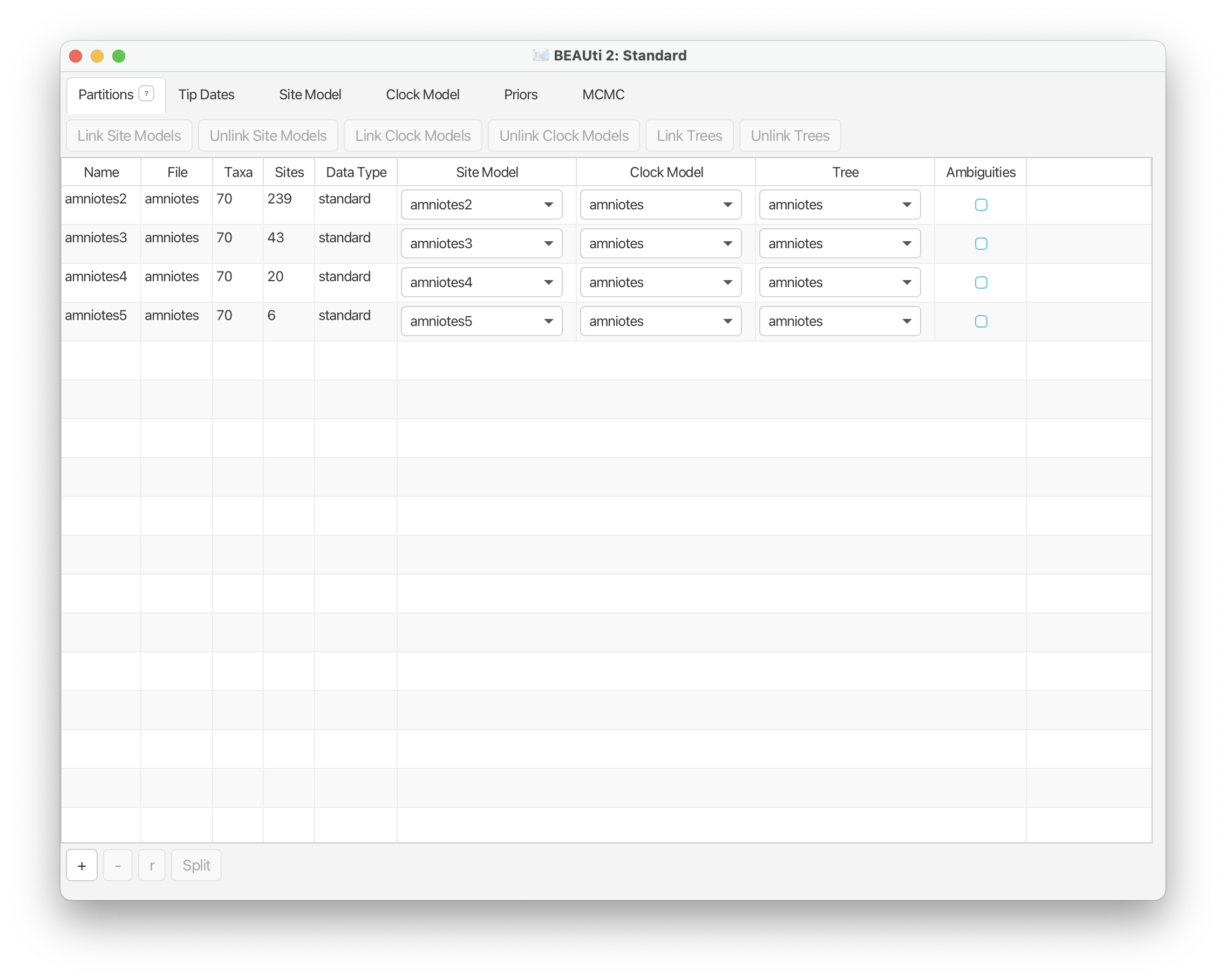
By default the characters are separated into four partitions. This means that characters will be assigned to a substitution rate matrix where the number of possible states corresponds to the maximum observed state for each character.
Note that the Site Model is unlinked across partitions, while the Clock and Tree models are linked by default. This means that we will allow each partition to evolve under an separate substitution process, but we will assume that the underlying tree is the same and that the same clock model is shared across partitions.
The Tip Dates panel
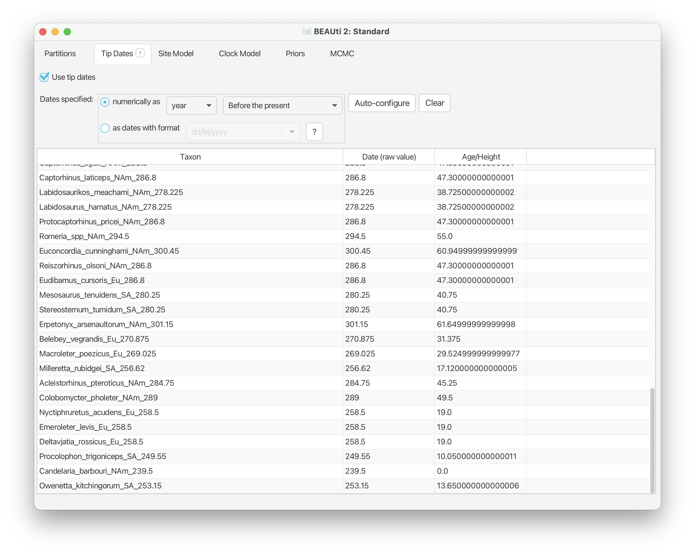
Navigate to the Tip Dates panel and select ‘Use tip dates’. Here we can extract information about the age of our samples from the tip labels. For our analysis, the time units are in millions of years, so we’ll leave ‘year’ selected in the first drop down menu. From the second drop down menu change ‘Since some time in the past’ to ‘Before the present’.
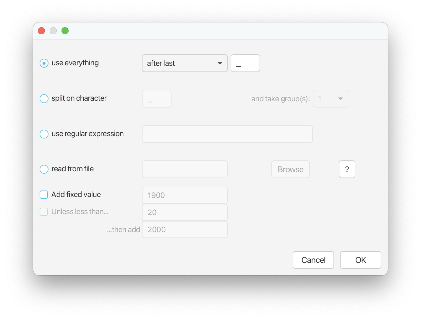
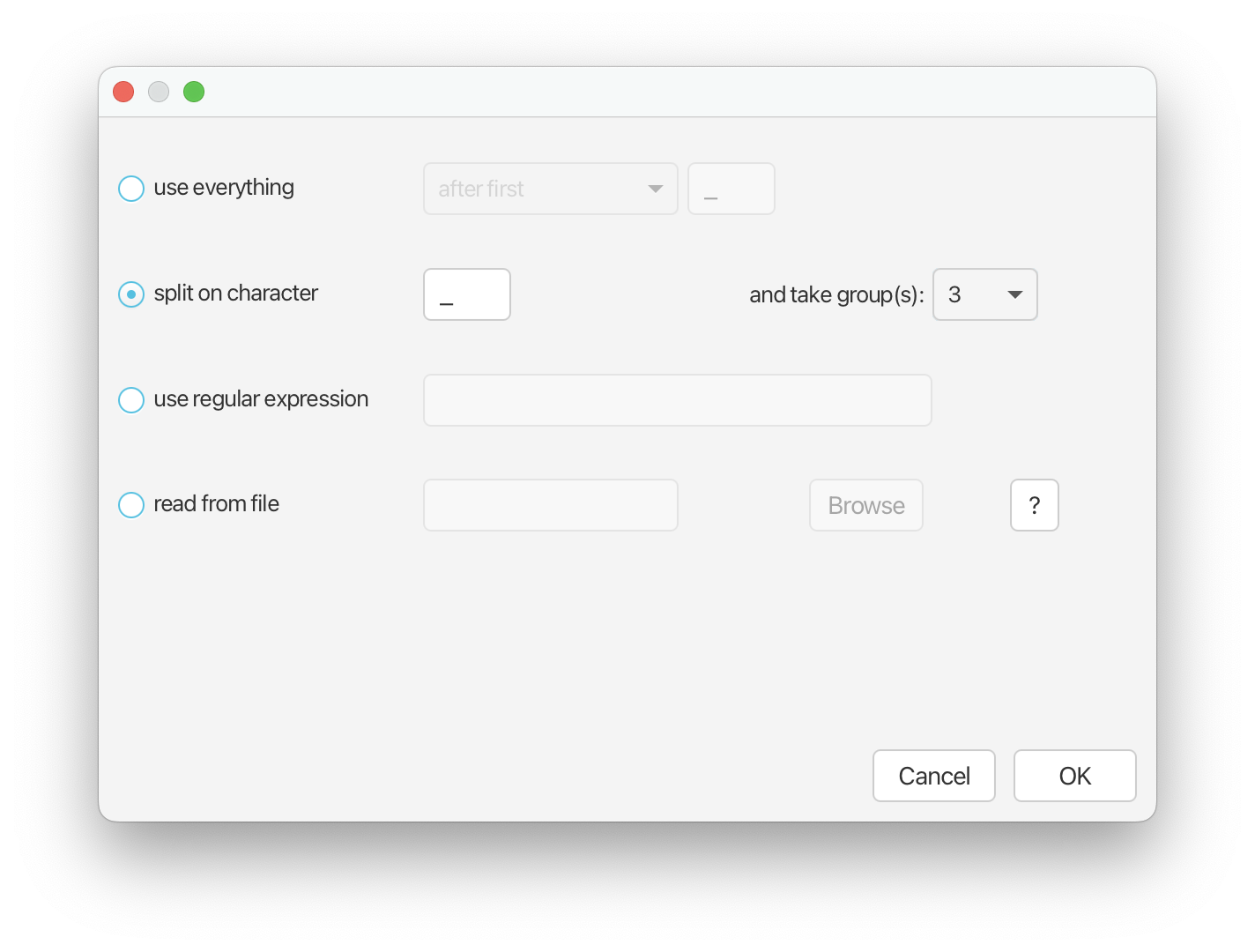
Next select ‘Auto-configure’. Leave ‘use everything’ selected and from the drop down menu select ‘after last’, leaving the delimiter as “_“. This will extract age information from the end of your taxon labels.
Note that although our samples span an interval in the past, internally BEAST rescales the tree such that the youngest sample in the tree is at t = 0. The rescaled values are shown under the Age/Height column.
To make sure everything is set up correctly, if you scroll down, the youngest fossil, ‘Candelaria_barbouri_NAm_239.5’, should have a “0.0” next to it under the Age/Height column.
The Site Model panel
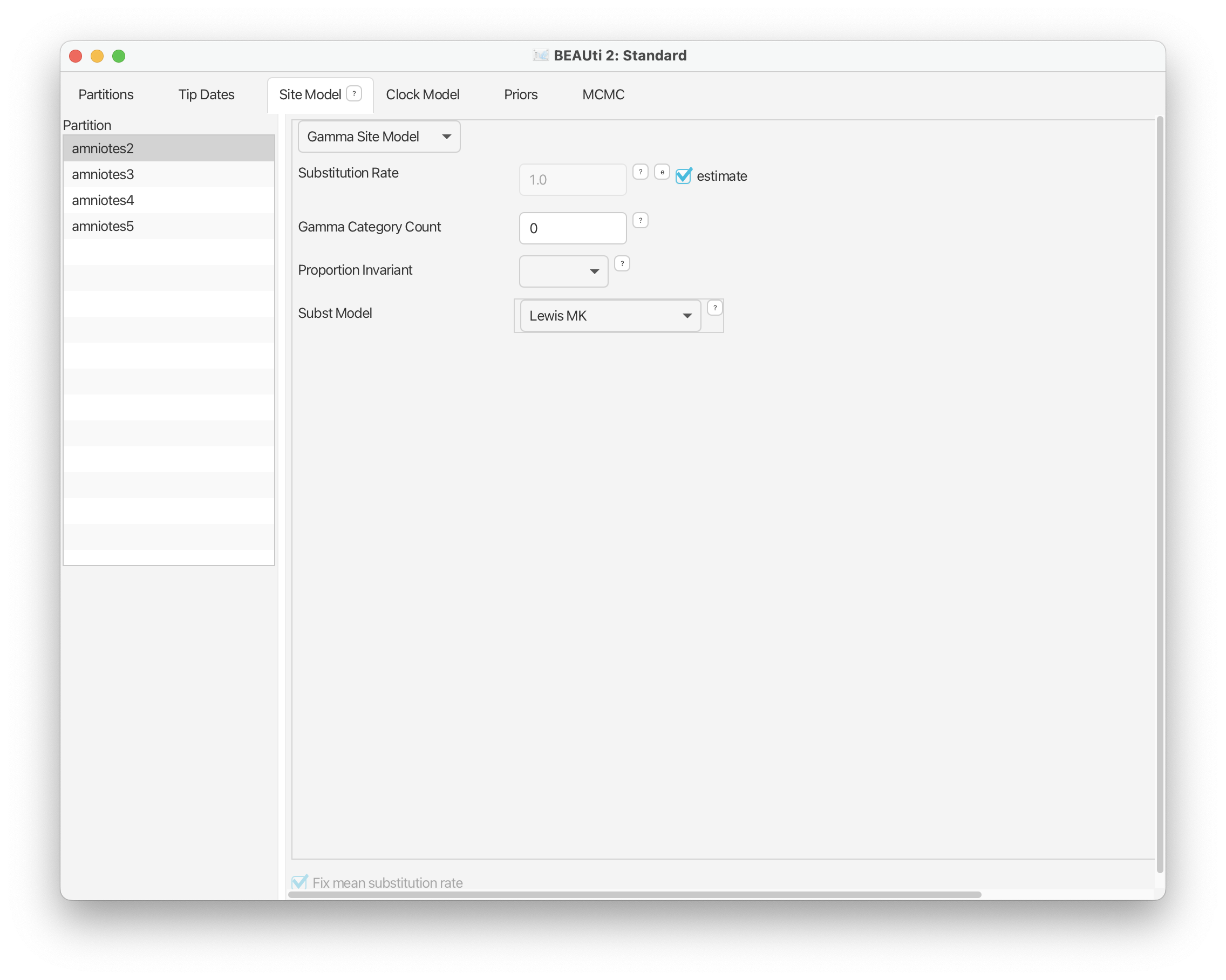
Under the Site Model panel we can specify the model of morphological evolution. For this exercise we’ll use the simple Mk Lewis model for each of our partitions and leave everything as it is.
The Clock Model panel
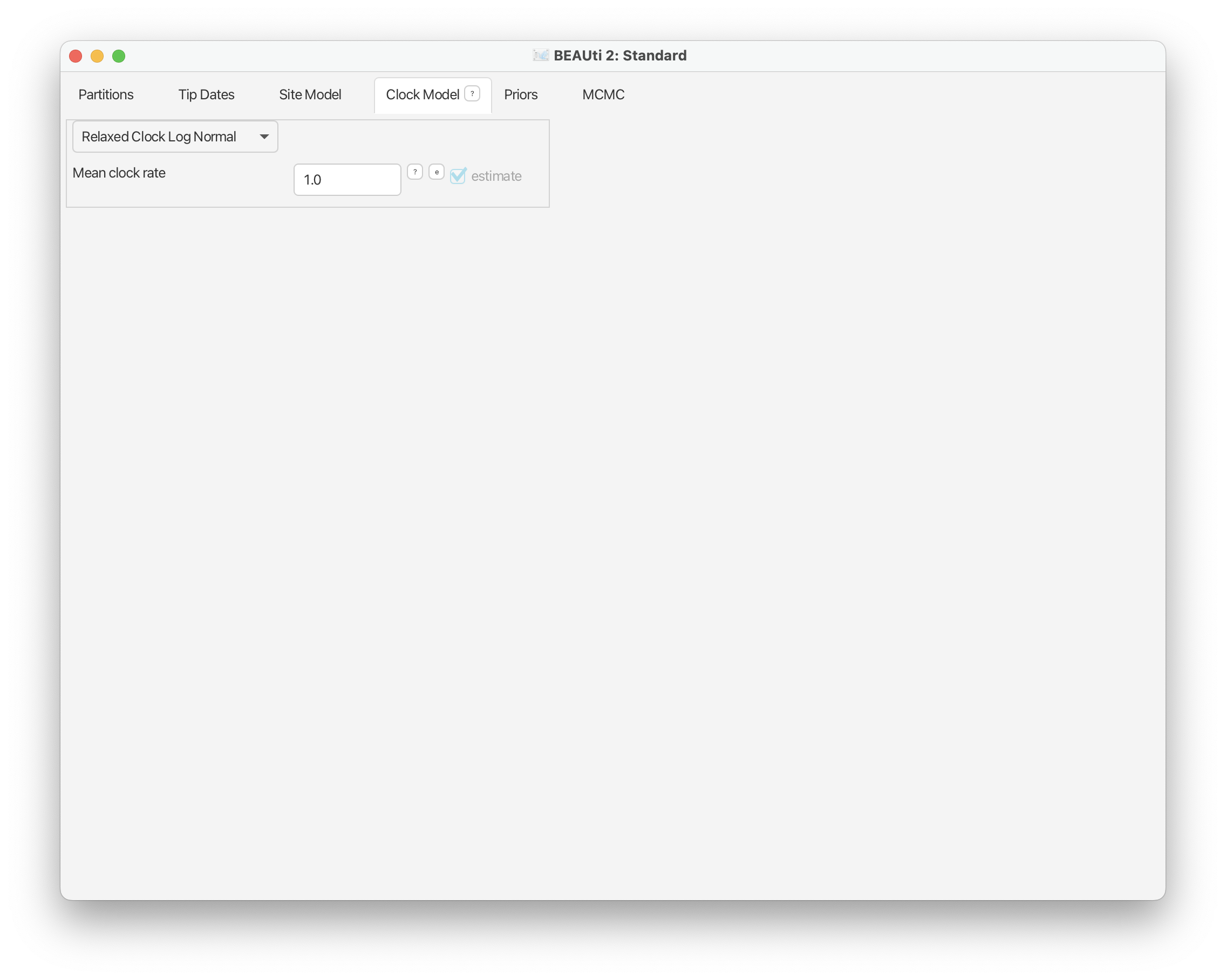
Navigate to the Clock Model panel and select ‘Relaxed Clock Log Normal’ from the drop down menu. This will allow rates of evolution to vary across branches in the our tree.
The Priors panel
Here we will set up the tree model and all the prior parameters associated with our analysis.
Clock model parameters
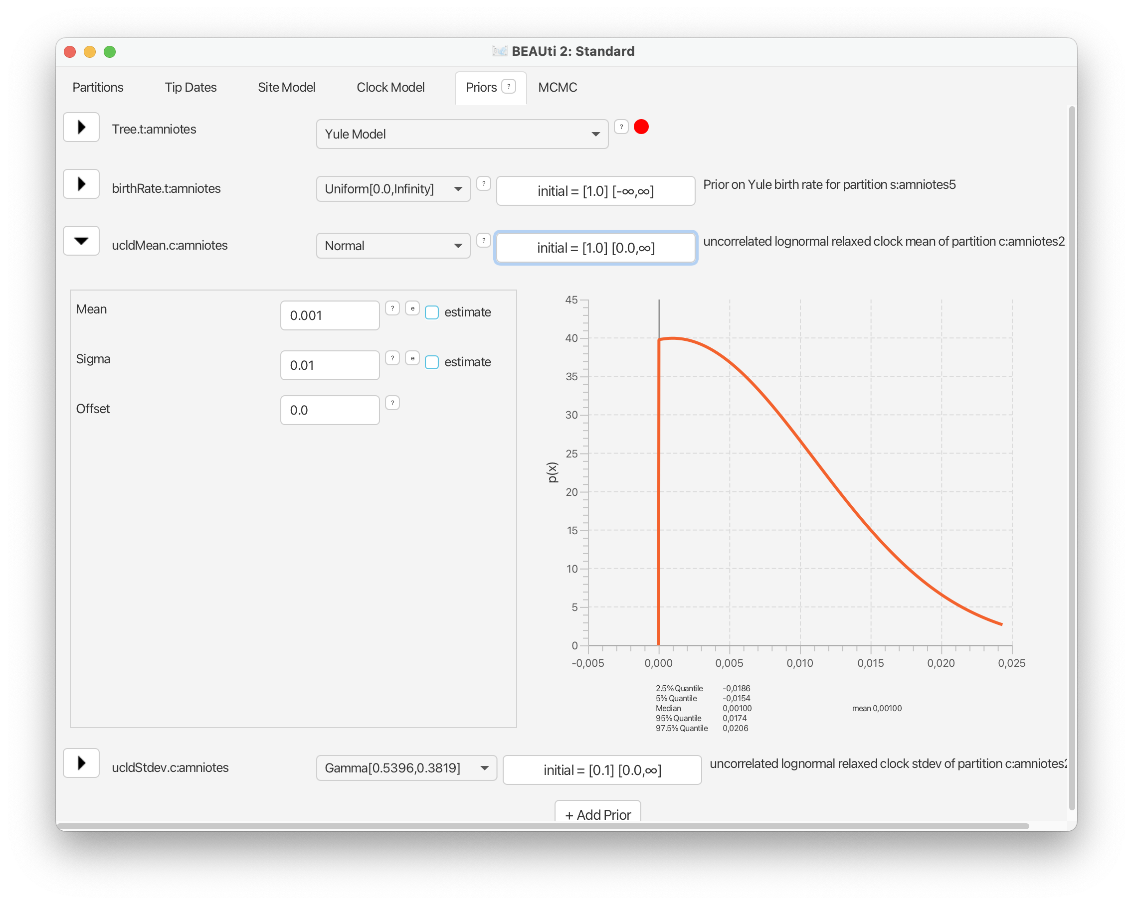
Let’s start with clock model parameters, ‘ucldMean’ and ‘ucldStdev’, which you should already see listed here.
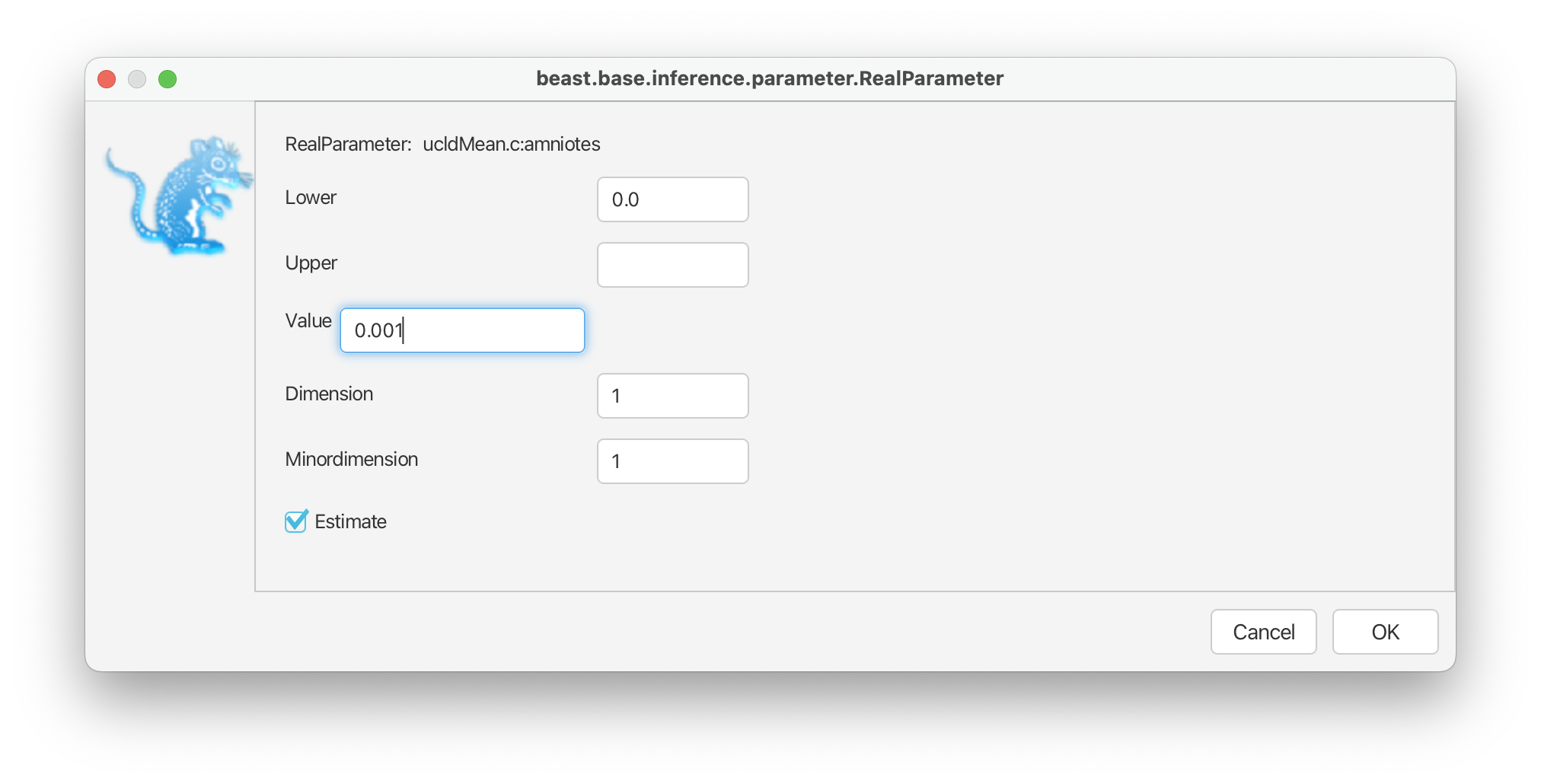
For the mean on the overall clock rate we will use a normal prior, following the original study, with a mean of 0.001 and a variance of 0.01. Note that rates cannot be negative so the distribution is truncated at zero. Finally, select the ‘initial’ value option next to the distribution and change ‘Value’ to 0.001. This ensures our analysis starts in a reasonable part of the parameter space. Click ‘OK’.
For the standard deviation of the distribution of clock rates, we’ll use an exponential prior with a mean of 0.1.
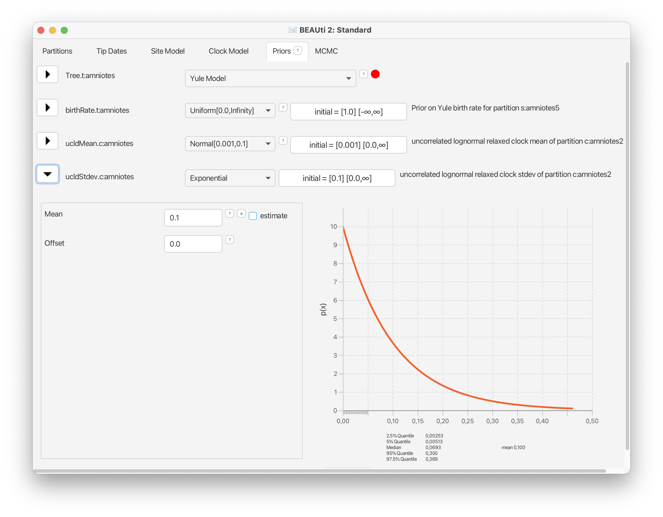
These prior choices match our expectations about rates of morphological evolution estimated in previous analyses of vertebrates, i.e., the rates tend to be relatively low, with some degree of variation across branches.
BDMM-Prime
Next let’s set up the phylodynamic model. Select ‘BDMMPrime’ from drop down menu at the top of the Priors panel.
There are a lot of options for combining parameters using BDMM-Prime, so we need to be careful to select parameter combinations that make sense for our dataset. There are three options for parameterising the birth-death model using BDMM-Prime. For macroevolution we can choose from two options:
- The “Canonical Parameterization”, which is parameterized using the birth (λ), death (μ), and sampling rates (ψ)
- The “Fossilized Birth Death Parameterization”, which is parameterized using diversification rate (d), turnover rate (v), and sampling proportion (s)
| Parameter | Transformation |
|---|---|
| Speciation (λ) | λ=d/(1−v) |
| Extinction (μ) | μ=(vd)(1−v) |
| Sampling (ψ) | ψ=(s/(1−s))((vd)/(1−v)) |
| Net diversification (d) | d=λ−μ |
| Turnover (v) | v=μ/λ |
| Sampling proportion (s) | s=ψ/(μ+ψ) |
The relationship between these parameters is shown in Table 1. Both are useful in macroevolution and your choice might depend on which parameters are of most interest to you or what prior information you have available. Note that after your analysis is complete, you can always go from one set of parameters to the other via the transformations shown in the table.
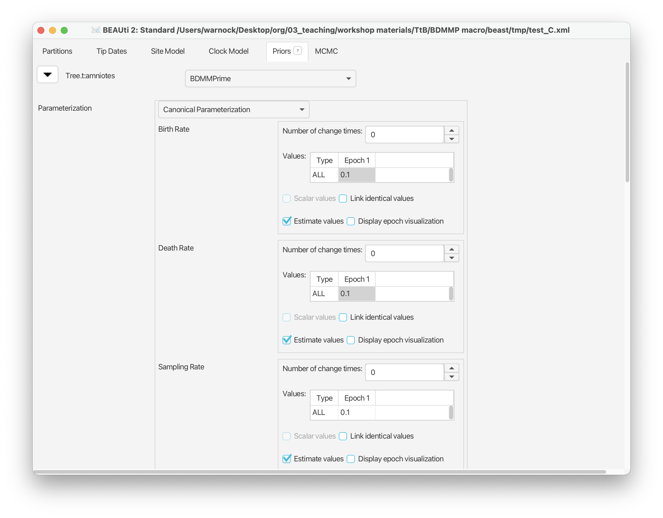
In this tutorial we’ll use the “Canonical Parameterization”, which you can select from the drop down menu next to ‘Parameterization’. This option can be applied to scenarios in both epidemiology and macroevolution.
Later we will assign taxa to types based on their geographic provenance but for the first analysis in this tutorial we’ll assume that birth, death, and sampling are all constant through time and across our tree. Thus we’ll leave “Number of change times” for each of these parameters as 0 (but see below). The only change we’ll make is to the value listed next to ‘Birth Rate’ and ‘Death Rate’ in Epoch 1, from 1.0 to 0.1 - these are the starting values for these parameters. Click on each value to edit it and press enter. Notice that ‘Estimate values’ is checked for all three of these parameters, which means these parameters will be estimated and not fixed during inference.
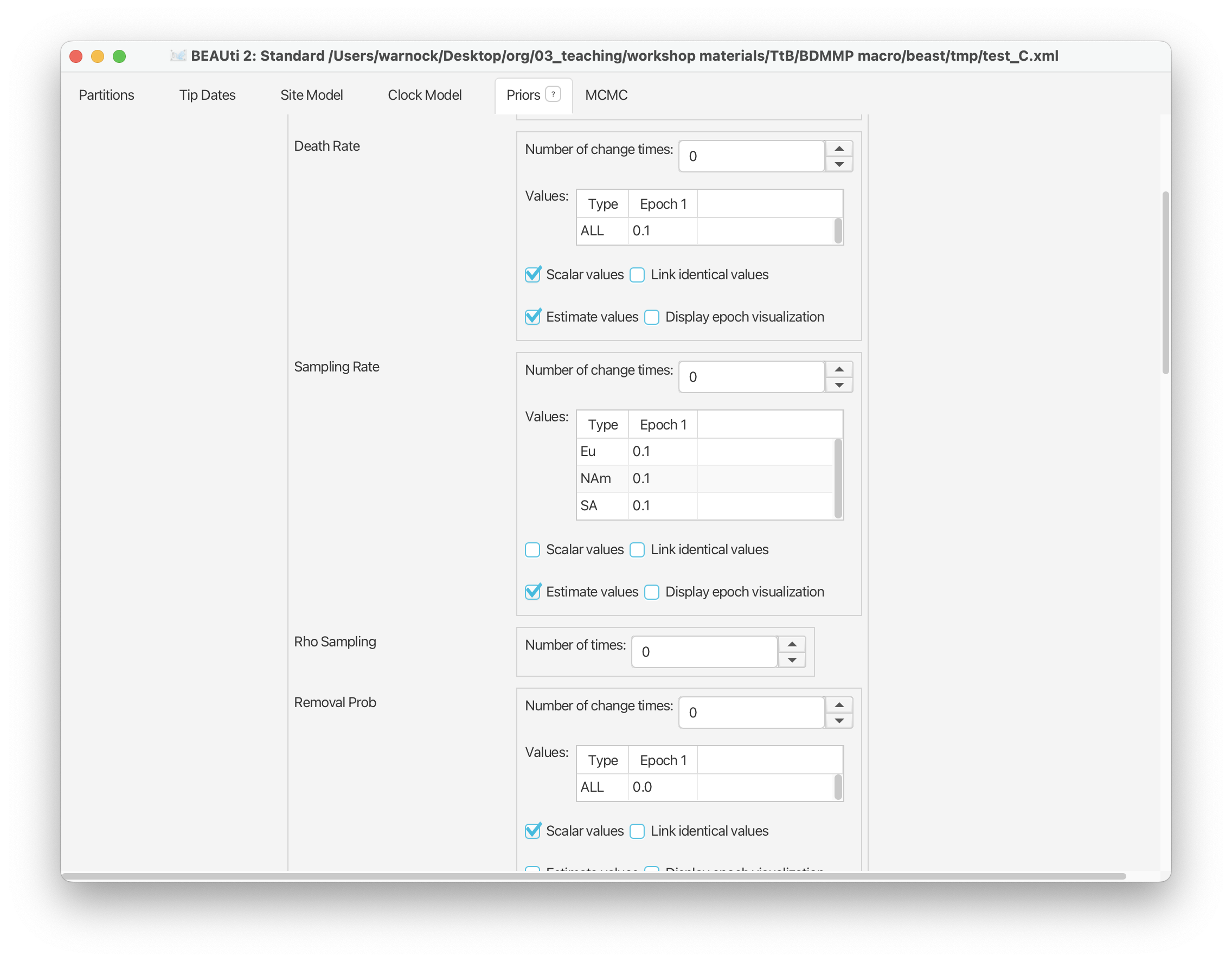
Scroll down to the next set of parameters of interest. ‘Rho Sampling’ is the probability of sampling a lineage at a given time. In macroevolution this is usually associated with the extant sampling probability at t = 0. In our case study, we have no sampling beyond the period of interest, i.e., the youngest sample included in our dataset is from the Triassic and is therefore ψ-sampled. There are many amniotes that persisted beyond this interval until the present but these are not included in our dataset. This means we have no rho-sampled taxa and it makes sense to leave Rho = 0.0.
The next parameter of note is the ‘Removal Prob’ - this is the probability that a lineage is removed from the population upon sampling and makes more sense in an epidemiological context. We need to change this to 0.0. Select the value listed next to Epoch 1 and change it to 0.0.
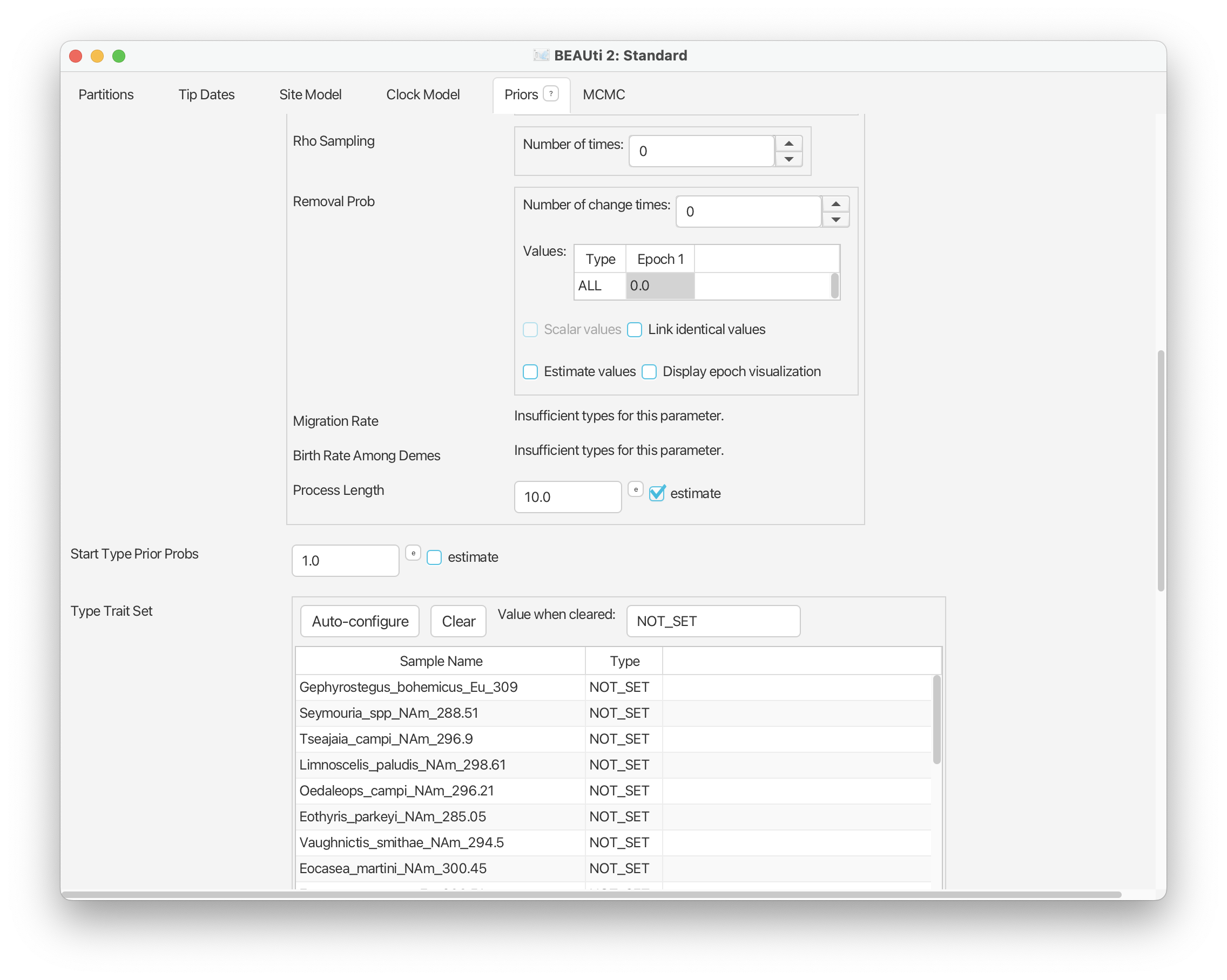
For now you can leave everything else under this tab as it is. If you close this tab and scroll down you should now be able to see an additional set of parameters listed in the Priors panel for the birth, death, sampling rates and the origin time parameter.
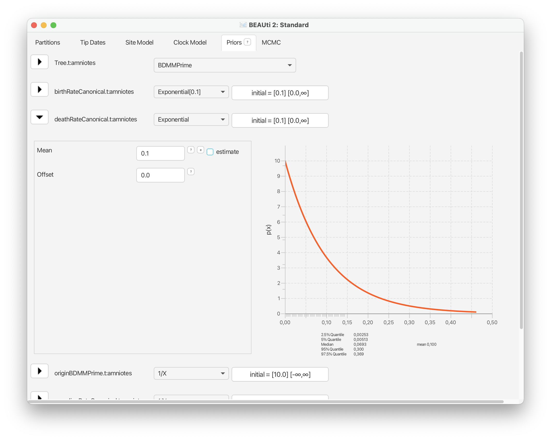
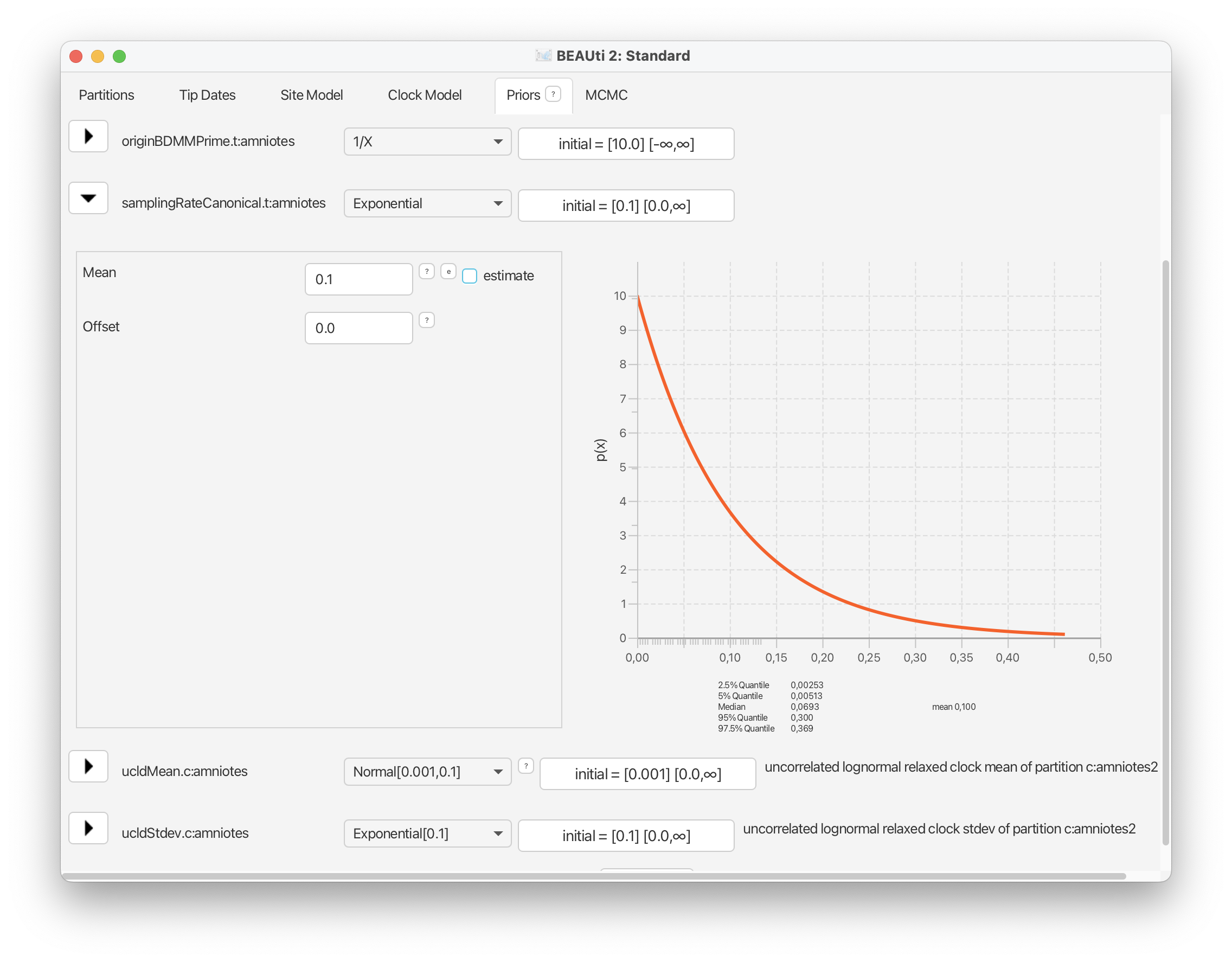
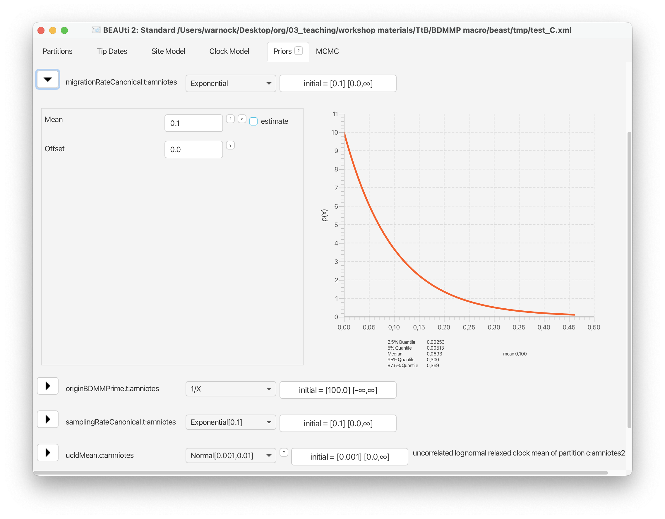
For the birth, death, and sampling rate parameters we’ll use an exponential prior with a mean = 0.1. This matches values that are typically estimated for these parameters in paleobiology.
From the drop down menu next to ‘birthRateCanonical’ select ‘Exponential’ and expand this selection. Change the mean of this distribution to 0.1.
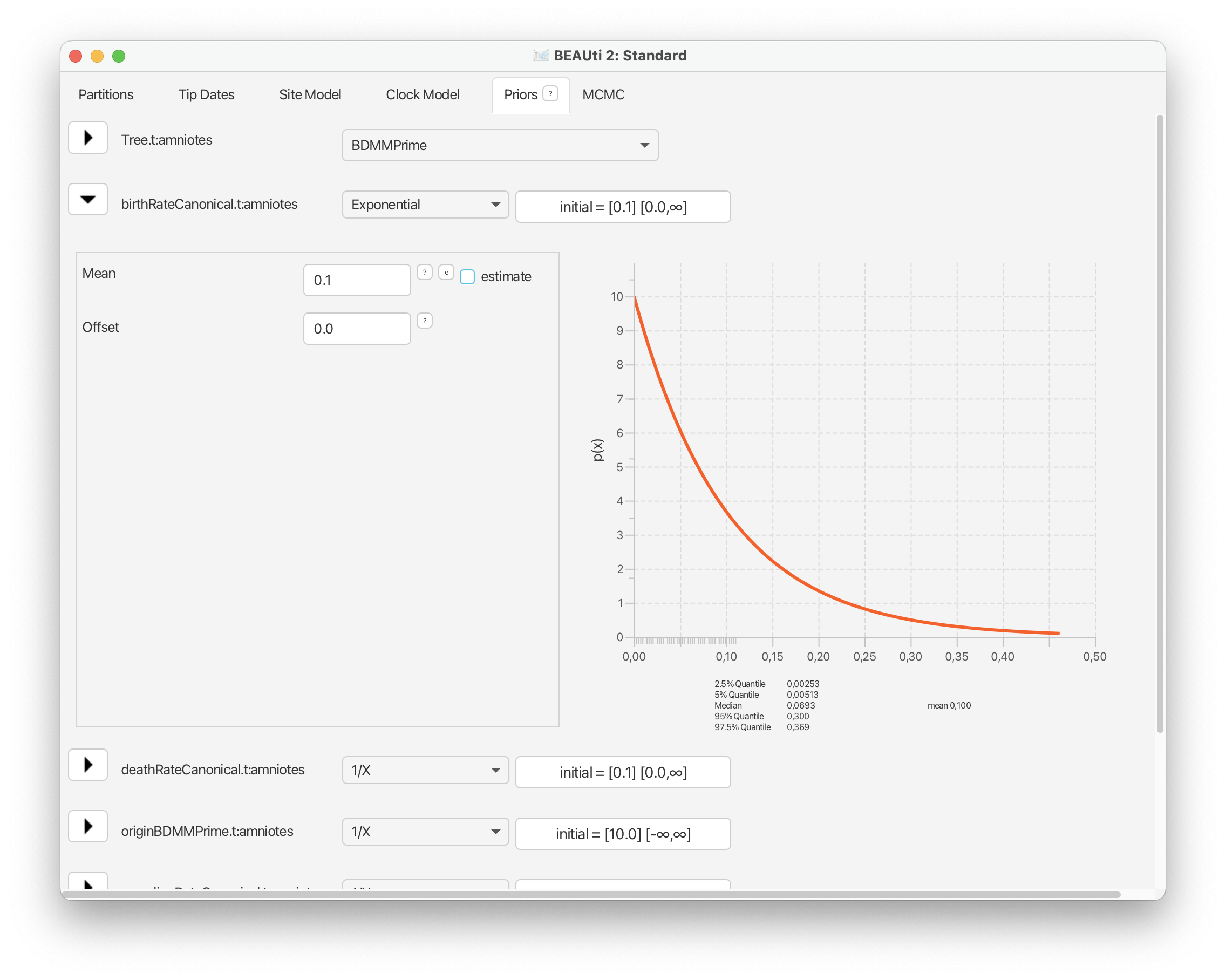
Go ahead and do the same for the death and sampling rate parameters.
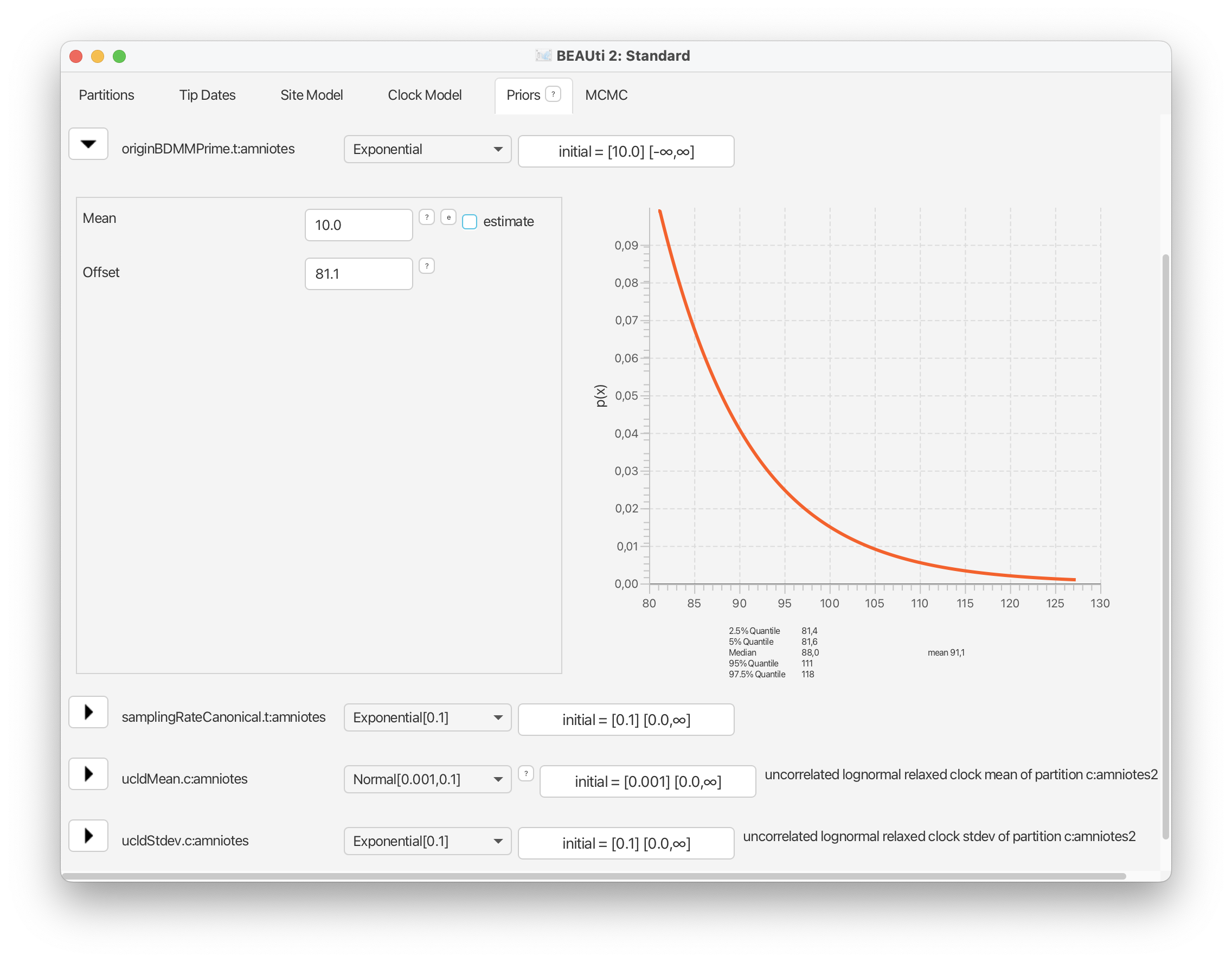
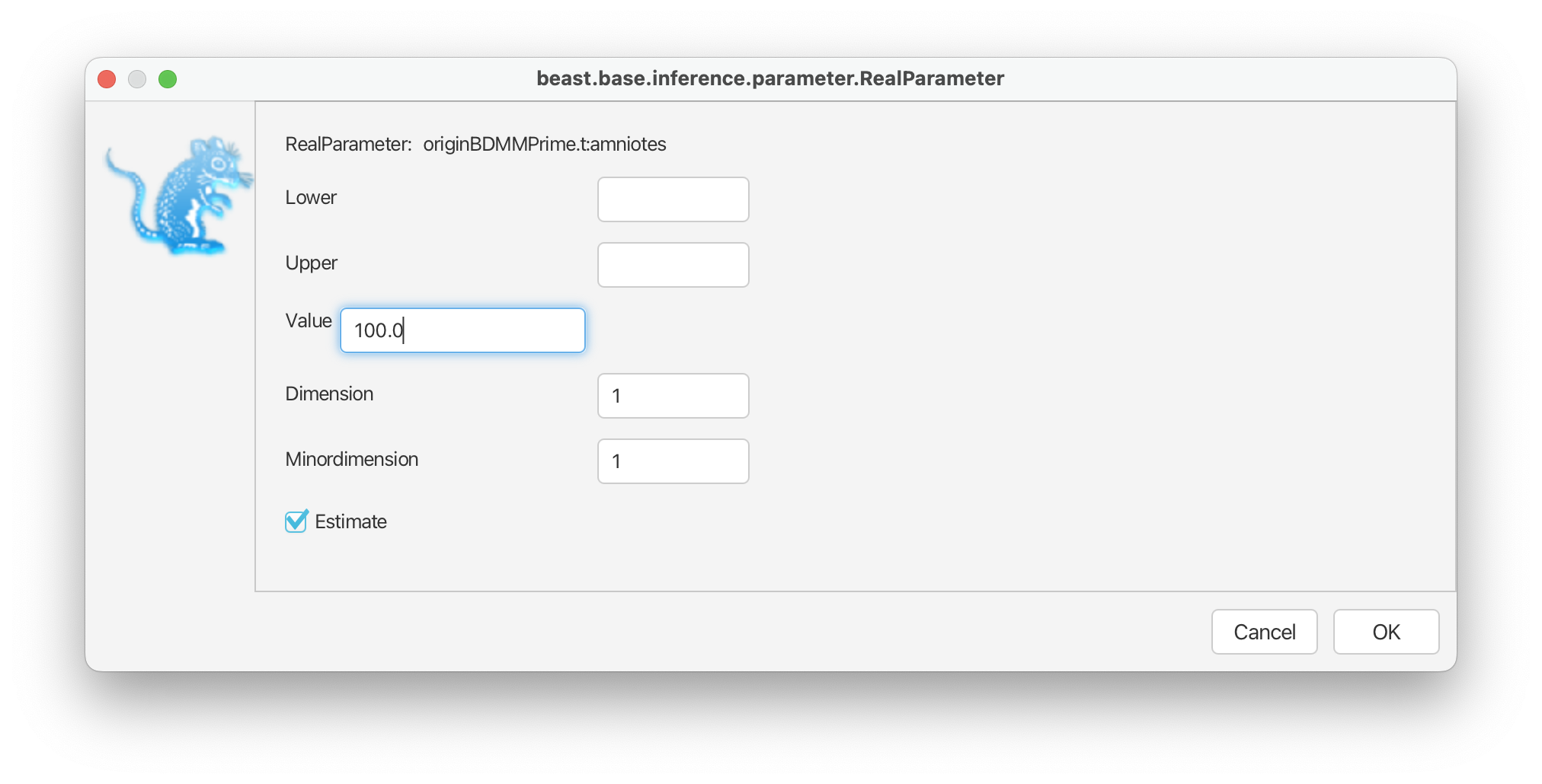
For the origin time parameter, we’ll also use an exponential distribution following the original study, with an offset = 318.1 Ma and a mean = 327.5 Ma. However, recall that BEAST scales the tree such the youngest sample is always zero, so these values need to be defined relative to t = 0. Select ‘Exponential’ from the drop down menu next to ‘originBDMMPrime’ and expand this selection. Change the offset to 81.1, which is 318.1 minus the youngest age of our sampling interval = 237, and change the mean to 10.0. Finally, select the ‘initial’ value box and change ‘Value’ to 100.0. The origin time of the process needs to be older than all our fossils. Click ‘OK’.
Adding taxonomic constraints
We’re going to use two taxonomic constraints for this analysis. Scroll down to the bottom of the Priors panel and click ‘+Add Prior’. From the drop down menu select ‘MRCA prior’. Click ‘OK’. This will open a box where you can define groups of taxa.
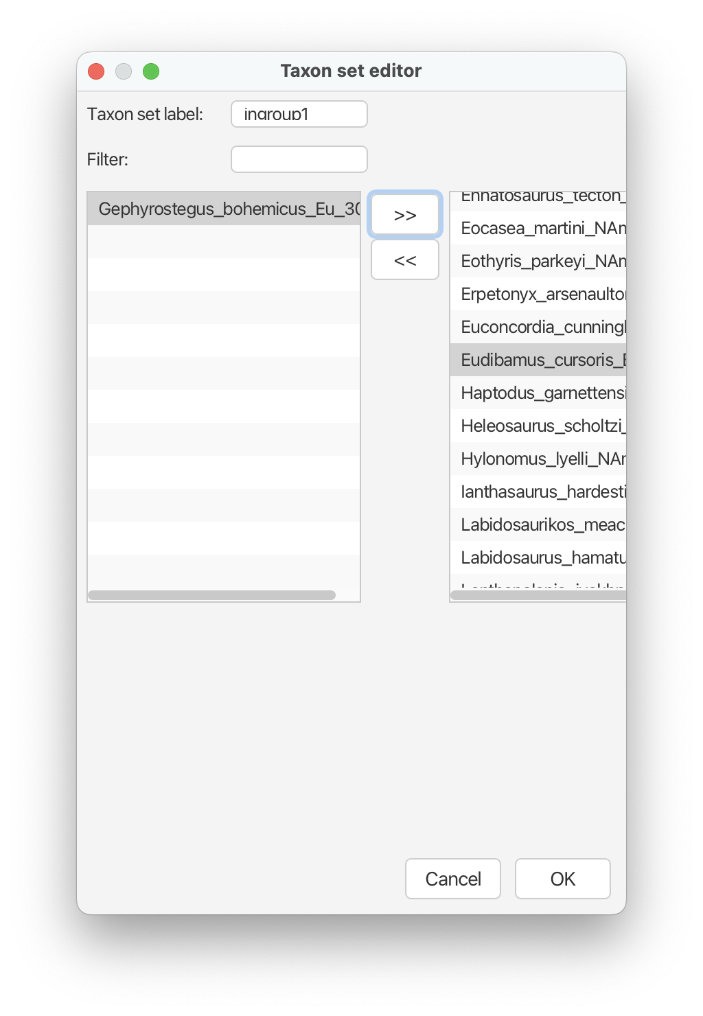
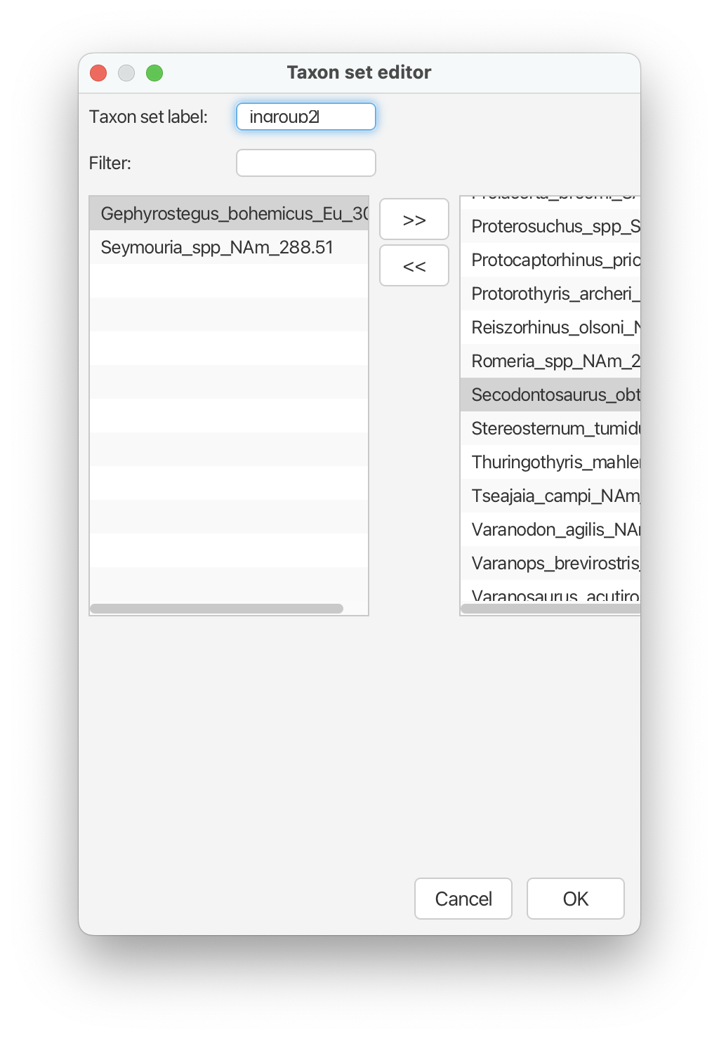
For the first constraint, type ‘ingroup1’ into the box next to ‘Taxon set label’. From the list of taxa on the left click on any taxa and use select all (e.g., cmd + A) to highlight all of them. Scroll down to ‘Gephyrostegus bohemicus’ and deselect this taxon using cmd + shift. Click the ‘>>’ button. Now all taxa except Gephyrostegus should appear on the right. Alternatively, you can select all of them, move them to the right and simply move Gephyrostegus back to the left using the ‘<<’ button.
Click ‘OK’ and then select the checkbox that says ‘monophyletic’ that appears next to this constraint.
To add the next constraint, click ‘+Add Prior’. From the drop down menu select ‘MRCA prior’. Click ‘OK’.
For the second constraint, type ‘ingroup2’ into the box next to ‘Taxon set label’. This next constraint will include all taxa except ‘Gephyrostegus bohemicus’ and ‘Seymouria_spp’.
 Click ‘OK’ and then select the checkbox that says ‘monophyletic’ that
appears next to this constraint.
Click ‘OK’ and then select the checkbox that says ‘monophyletic’ that
appears next to this constraint.
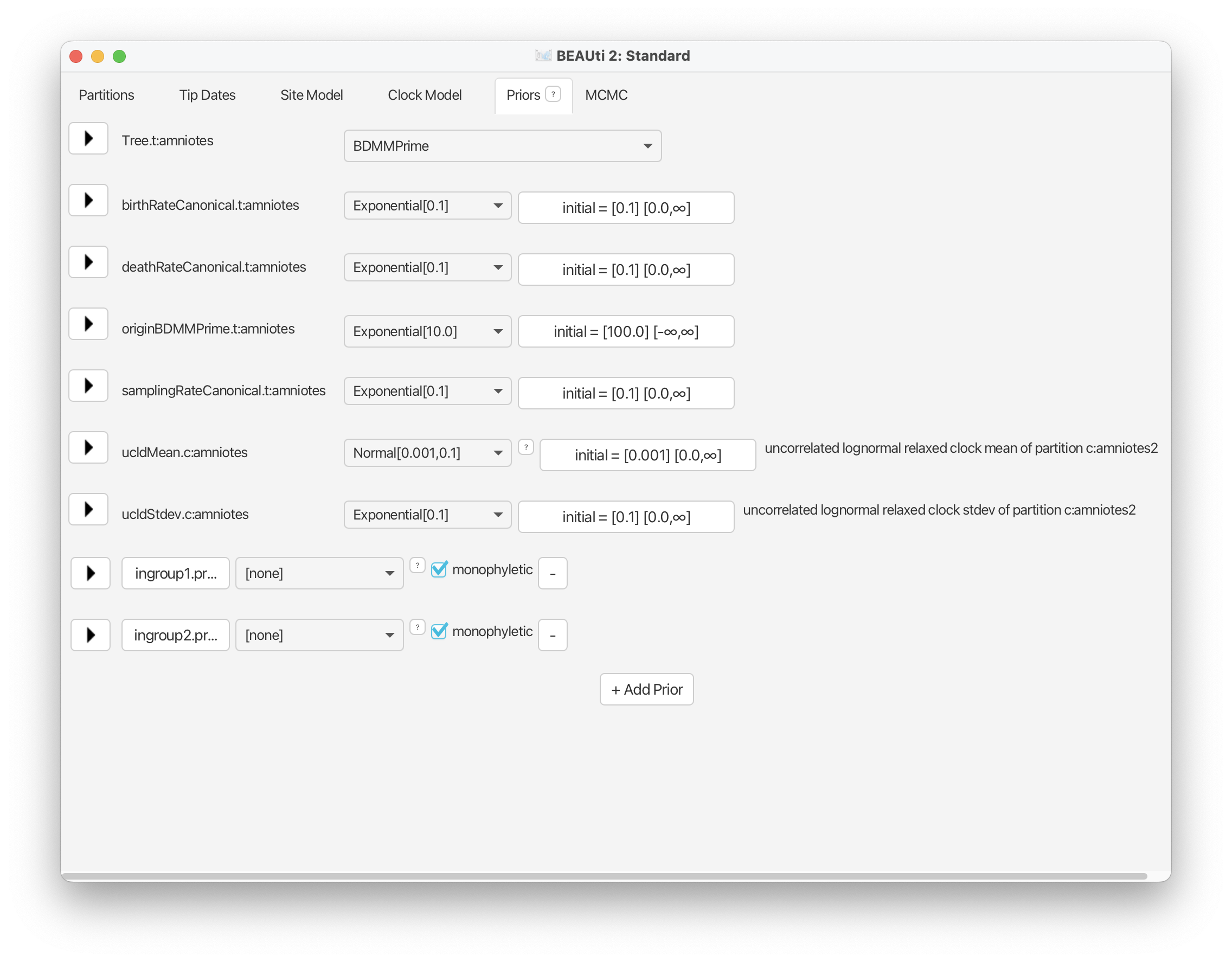
Use this screen shot to ensure all your prior distributions and initial values have been set up as described.
The MCMC panel
Navigate to the MCMC panel. For now, we’ll leave all the MCMC settings as the defaults.
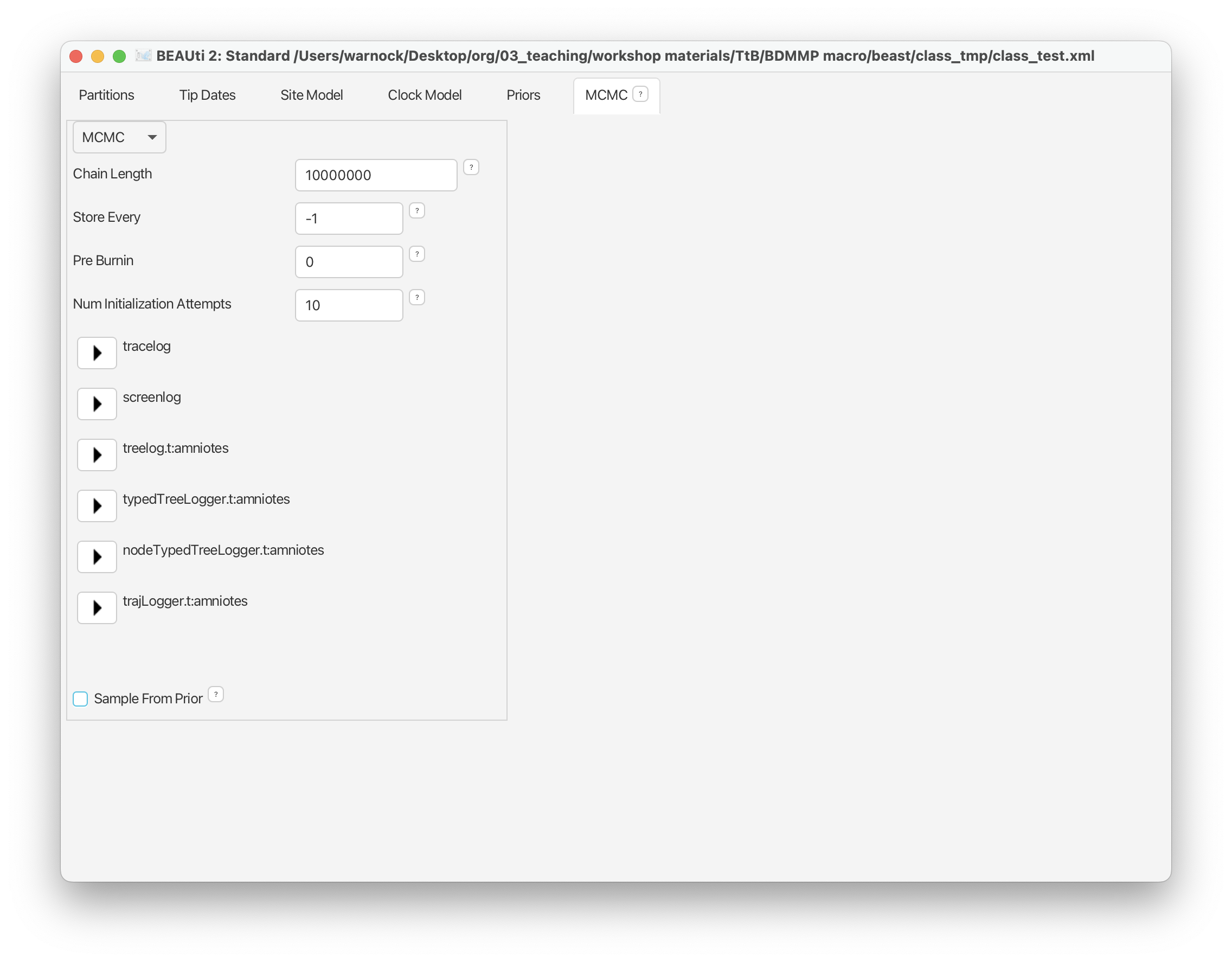
Go to ‘File > Save as’ to save your xml input file. Call it something like ‘amniotes_constant_rates_FBD.xml’ or anything you like.
You can leave BEAUti open for the next part of the exercise! However, if you do close BEAUTi you can simply go to ‘File > Load’ and select your xml file - all the BDMM-Prime specifications should be reloaded.
Running BEAST
To run your analysis open the BEAST application and navigate to the right working directory. Select your xml file and click ‘Run’.
This analysis should take ~10-15 minutes to run. While your analysis is running you can move on to part 2 (the multi-type birth-death process).
Examining the output
First open the .log file in Tracer and explore the output. It should look something like this.
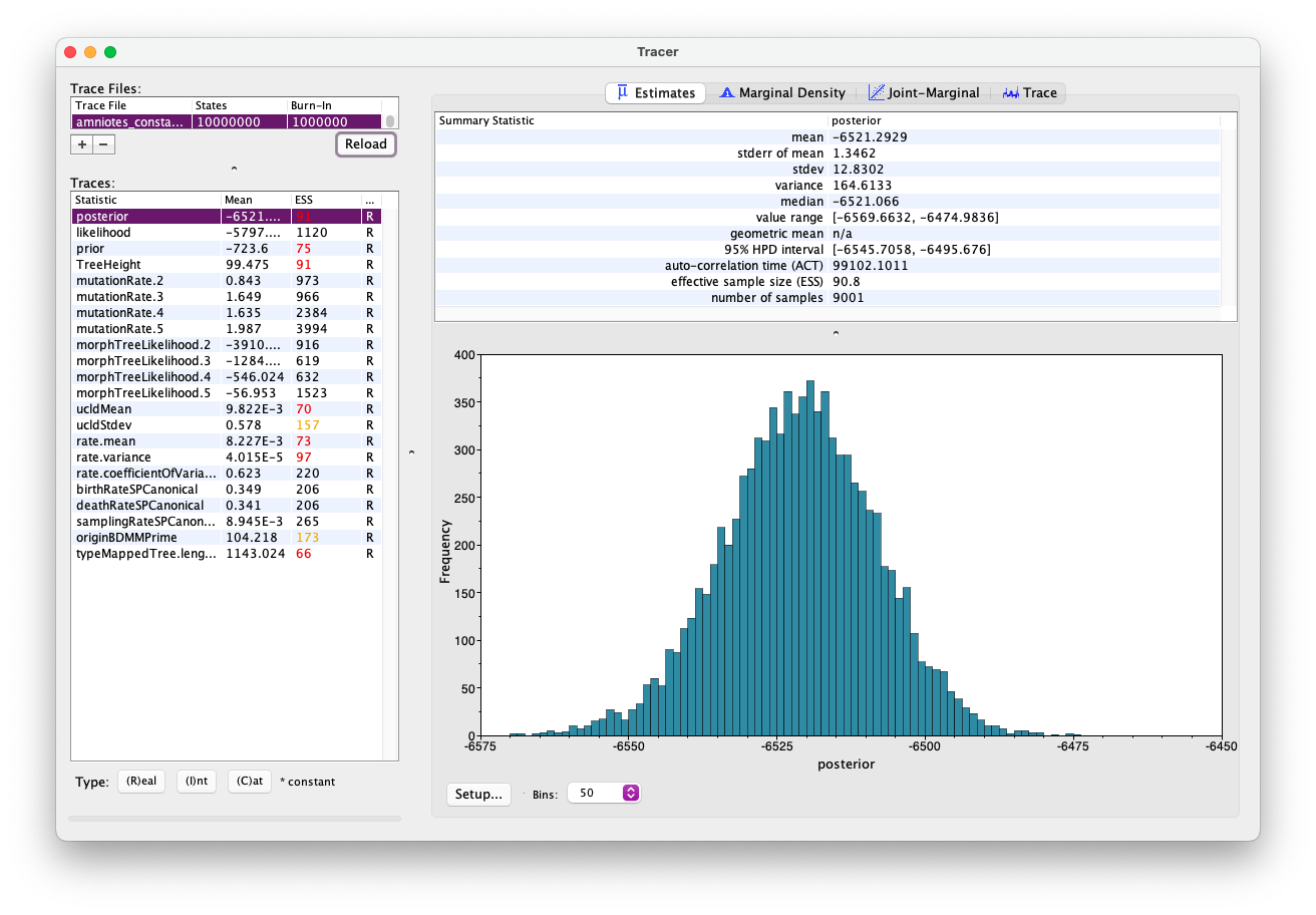
Of particular interest are the parameters ‘birthRateSPCanonical’, ‘deathRateSPCanonical’, and ‘samplingRateSPCanonical’. The speciation and extinction rates are both ~0.35, while the sampling rate is ~0.01. This suggests that sampling is low relative to the overall diversity of the group.
Note that this analysis hasn’t fully converged but you can download the pre-cooked output for the same analysis that’s been run a bit longer.
If you want you can also generate a consensus tree using the standard .trees file (‘amniotes.trees’) and the approach described in previous tutorials for trees with sampled ancestors. For the ‘Target tree type’ stick with the default ‘Maximum clade credibility tree’ and for the ‘Node Heights’ select ‘Median heights’ from the drop down menu.
The multi-type birth-death process
Create a new folder to run this next analysis.
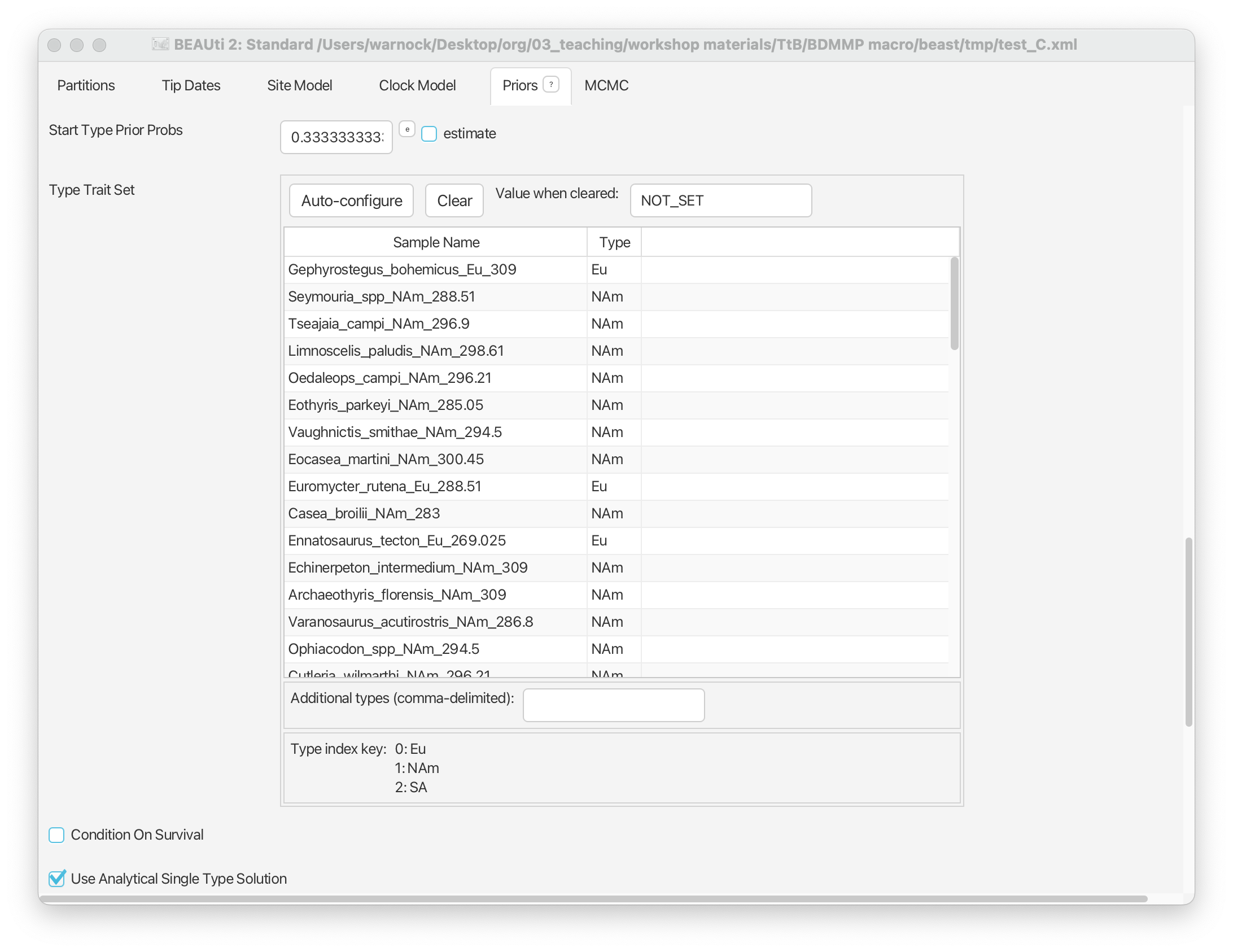
Return to the Priors panel in BEAUti. Next we’re going to add information to the analysis about geographic area. Expand the tree model selection and scroll down to ‘Type Trait Set’. Click Auto-configure. Select ‘split on character’ and from the drop down menu next to ‘and take group(s):’ select 3.
Click ‘OK’. You should now be able to see the geographic area associated with each fossil in the ‘Type’ column (Eurasia, North America, and South Africa).
Scroll up and you should see some additional options have been added for the tree model. In particular, options will have been added for the ‘Migration Rate’ and ‘Birth Rate Among Demes’ parameters. The migration rate can be interpreted as the rate of change between types (in our case, geographic areas). We’ll estimate this parameter and leave the settings as they are here. The birth rate among demes can be interpreted as the rate of “spontaneous” change between types - in epidemiology this might be used together with types that are associated with specific mutations. This parameter doesn’t have an analogous meaning in our macroevolutionary context, so we’ll simply fix this parameter to zero.
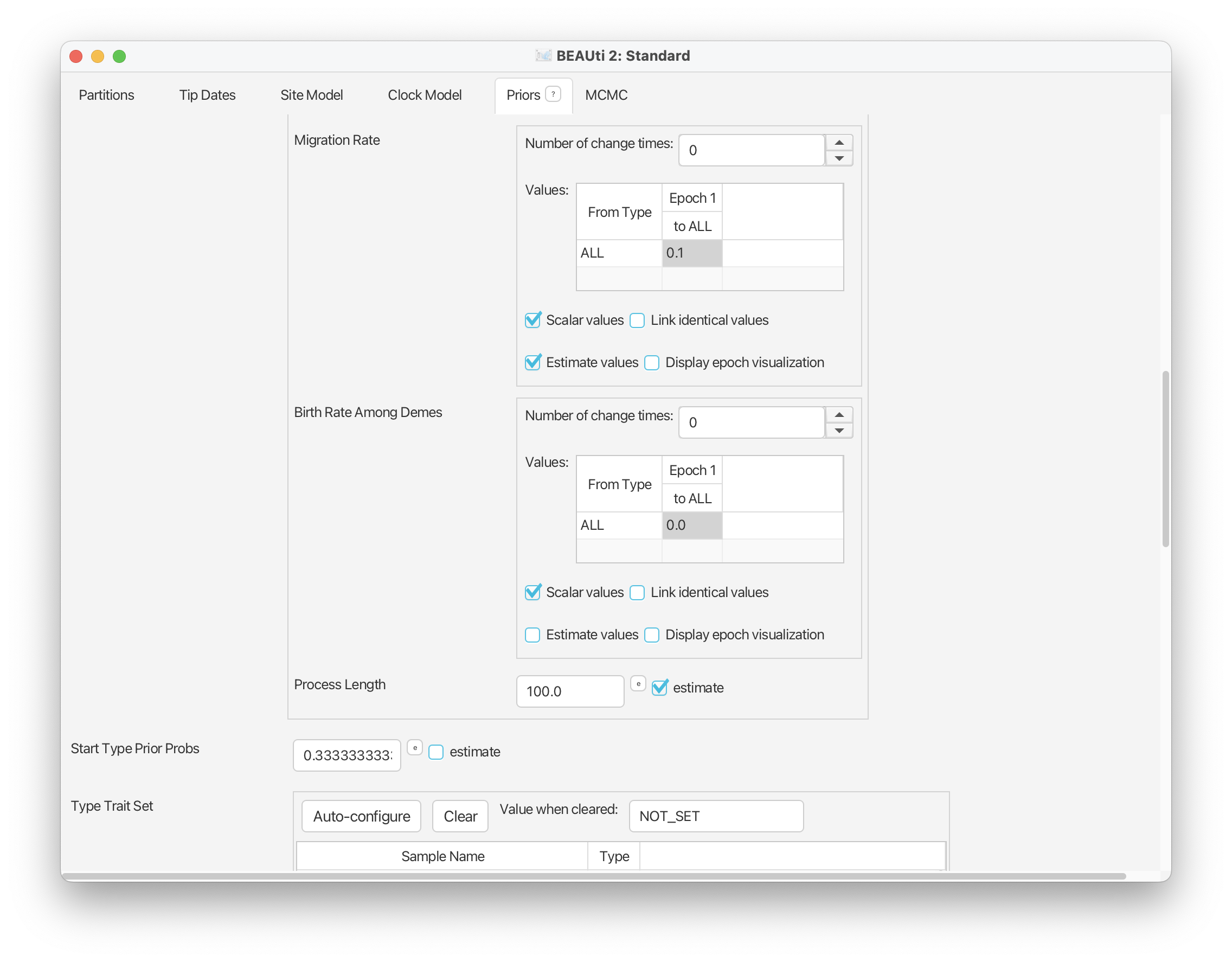
In this analysis we want to allow sampling to vary across geographic areas. To do this scroll back up to the tree model options. You’ll see that next to each parameter is a checked box called ‘Scalar values’ - this indicates that a single rate applies to all types. If you uncheck this box a separate rate will be applied to each type - in our case, each geographic region.
TODO Note that we can define the Start Type Prior Probs. By default… This probability can be estimated but we’ll leave this as it is.
Finally, scroll down and assign an exponential prior to the migration rate parameter.
Navigate to the MCMC panel and change the ‘Chain Length’ to 1,000,000 (just delete one of the zeros).

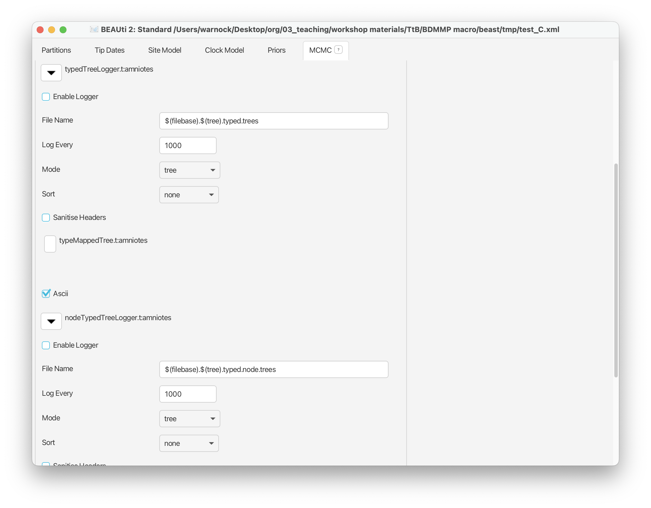
We’re also going to switch off the ‘typedTree’ and ‘nodeTypedTree’ loggers - find these options and uncheck ‘Enable Logger’.
Go to ‘File > Save as’ to save your xml input file in your new folder. Call it something like ‘amniotes_multi_type_FBD.xml’.
You can leave BEAUti open for the next part of the exercise!
Running BEAST
As above, run your analysis open the BEAST application and navigate to the right working directory. Select your xml file and click Run.
This analysis should take ~15 minutes to run. Ideally this analysis would run for much longer, e.g., 10,000,000+ generations, but this takes about 8 hours!!
Examining the output
Open the .log file in Tracer and explore the output. It should look something like this.
Now we have some additional parameters of interest. In particular, we have three estimates for ‘samplingRateSPCanonical’ associated with each type or geographic region. Select all three sampling values and compare them. You should be able to see that the median estimate is slightly higher for North America, followed by Eurasia and South Africa, which matches our understanding of how intensively each of these regions have been sampled.
If you scroll down you should also be able to see estimates associated with the transitions between each type. The ‘typeMappedTree.length’ variables tell us how much of the total tree length is associated with each region, while the ‘typeMappedTree.count’ provides a posterior estimate for the number of migration events between each region along our sampled tree.
At the bottom we also find an estimate for the ‘migrationRateSPCanonical’ parameter.
- TreeAnnotor
The skyline birth-death process
As above, create a new folder to run this next analysis.
Return to the Priors panel in BEAUti. Next we’re going to allow birth rate and death rate to vary over time. Locate the options associated with ‘Birth Rate’. Change ‘Number of change times:’ to 2. Select ‘Relative to process length’ and click ‘Distribute evenly’ - this means that the time between the origin of the process and the end will always be divided into 3 equal intervals and each one will be assigned an independent rate parameter. You can select ‘Display epoch visualisation’ to make sure things are set up correctly.
Do exactly the same for the ‘Death Rate’.
Note that BEAUTi will assign the same prior to the rates in each interval. In our case, this means that for each interval the birth and death rates will be drawn from a separate exponential prior distribution.
Go to ‘File > Save as’ to save your xml input file. Call it something like ‘amniotes_multi_type_skyline_FBD.xml’.
Running BEAST
As above, run your analysis open the BEAST application and navigate to the right working directory. Select your xml file and click Run.
This analysis should take ~15 minutes to run. Ideally this analysis would run for much longer, e.g., 10,000,000+ generations, but this takes about 8 hours!!
TODO Examining the output
- log file
Compare the log files obtained using different parameter combinations. What conclusions can you draw?